- This topic has 17 replies, 7 voices, and was last updated 3 years ago by Killer.
-
Excel wizards help please!
-
richardkennerleyFull MemberPosted 3 years ago
Trying to compile some data at work but i’ve reached a point where it’s beyond my skills!
 [/url]” alt=”excel” />twistyFull MemberPosted 3 years ago
Keen to help but need a bit more of a steer on what you need solving 🙂
richardkennerleyFull MemberPosted 3 years agoBloody computer just logged me out and restarted!
Bear with me
richardkennerleyFull MemberPosted 3 years agoOk
Column B show sample number
Column F shows tests carried out on the sample, column G shows the corresponding result for each test.
There’s usually 5 tests (sometimes more) for each sample, so for each sample there’s 5 rows.
I need the tests in F to form new columns with headers and the results in G to show in the correct column all on one line for each sample number in B.
Does that make sense!?
richardkennerleyFull MemberPosted 3 years agooo, that worked a bit better!
So you can see the tests in column F need to form new column headers
URBC UPOL UEP YEA ORG
Then the corresponding result from column G dropped into the right place along one line for each sample number of column B
polyFree MemberPosted 3 years agoIt sounds like all you need is In H1 to L1 put each of the test types URBC etc.
Then in H2:
=if($f2=h$1,G2,)
Then drag fill across the columns and down the rows.
twistyFull MemberPosted 3 years agoThe easy way of doing this is adding the columns to the list for each test type and then using some if statements to populate the value if it is that type of test (example below).
The more elegant way is to use a formula in a seperate sheet (which can be a template of sorts) to display a filtered list, and then look up and populate the values for each test type if they are there, but I don’t quite have time to work through that solution right now.
https://drive.google.com/file/d/1FIvuFTyXCdCAKFs7c4retBufTP8fcuhD/view?usp=sharing
GreybeardFree MemberPosted 3 years agotwisty’s first solution works if there’s a fixed number of rows for each lab number. The difficulty is that the number of rows isn’t always 5, so the position of each test result isn’t fixed relative to the first row. You can’t simply use VLOOKUP to find the result for each test as you’ll have to set the lookup range to allow for the maximum number of rows for any lab number, so in some cases you’ll catch the results for the next lab number. I would try adding a temporary column containing a concatenation of lab number and test. Then you can use twisty’s approach and reference column B concatenated with the column heading and do VLOOKUP on that unique value.
joshvegasFree MemberPosted 3 years agoUnless i have the wrong end of the stick thats got pivot table written all over it.
polyFree MemberPosted 3 years agoOh, I just read the bit about wanting all identical sample numbers on one row. You can probably do what I suggested and then add a pivot table. Vlookups are good if the data is guaranteed to be structured a particular way… of course this is yet another example of someone using excel for something which it really isn’t great for – and it would be better investing a day in learning a basic level of software/data analysis like python to do it properly (where at least erroneous data will be labelled as such).
richardkennerleyFull MemberPosted 3 years agoof course this is yet another example of someone using excel for something which it really isn’t great for – and it would be better investing a day in learning a basic level of software/data analysis like python to do it properly (where at least erroneous data will be labelled as such).
Ha. What it actually is is an example of how the NHS works… expect someone with no experience and non of the correct tools to just work out how to do something or resort to asking a mountain biking forum for help.
I’m a trained microbiology biomedical scientist. I have no data analysis skills or training and access to Excel and Access and nothing else.
Thanks for the help so far, I tried the formula suggested above, I can see how that should work but it only works on the one cell I apply it to, it doesn’t drag and populate the rest of the table.
dc1988Full MemberPosted 3 years agoIf you have a list of number going down and you just need them to go across then you can do paste special transpose, don’t know if this might help you.
joshvegasFree MemberPosted 3 years agoYou could use an array formula to reduce tje test numbers to one row for each.
Then you can use a concatenation formula of test number & test results from the entries against new rows and column headings.
Um. I think thats what you can do but its been a while and i am trying to teach myself steel structure design basically in a day.
polyFree MemberPosted 3 years agoHa. What it actually is is an example of how the NHS works… expect someone with no experience and non of the correct tools to just work out how to do something or resort to asking a mountain biking forum for help.
mmm… yes I know your problem well, and right up until someone gets the wrong result because someone put a space after the characters with the test type it all seems great. For reasons I’ve never understood there is no requirement for you to validate your spreadsheet actually works!
I’m a trained microbiology biomedical scientist. I have no data analysis skills or training and access to Excel and Access and nothing else.
It’s actually a failing of education as much as your employer. Vocational training institutions should know that increasingly people like you will be asked to do things like this and equip you with the skills. However next time you get asked in an appraisal if you have any training needs – tell them you want some training in data analysis tools. Python and R (depending exactly what you are doing) are free – so you are talking about some online training, or a one/two day workshop. If you worked for me and had shown an actual interest in this (eg by doing some free online learning) I’d be biting your hand off to send you to something like the Edinburgh Uni “data carpentry” course (I think there is funding available for that so just your time).
Thanks for the help so far, I tried the formula suggested above, I can see how that should work but it only works on the one cell I apply it to, it doesn’t drag and populate the rest of the table.
OK I have no idea how skilled you are in Excel. I’m going to assume not. So when you say doesn’t drag and populate to the rest of the table – do you mean you don’t know how to fill down and fill across? If that’s the case I am guessing you don’t know the significance of the $ signs in the formula? I’m not sure I’m comfortable providing Excel help for a medical related solution where the risk of error could be high and the user is unlikely to spot it easily. However, if you want to copy a formula down you can select a cell and then drag the bottom right of that cell down or across. It’s Vaguely intelligent so tries to assume That you want the cells it points to to change as well but sometimes you don’t – and so the $ sign comes in handy. If this is news to you search YouTube For FillDown Excel and you should find something. If I’ve just patronised the hell out of you, apologies, but tell us more about what you couldn’t do.
Now you probably want to find a tutorial on Pivot Tables. BUT be warned they are not fun, and if you appear to be competent at them everyone in your department will come to you for all excel needs forever.
joshvegasFree MemberPosted 3 years agoPivot tables are fun ignore poly.
But as Poly alludes to… Tell no one.
My approach fleshed out a little would be.
New column in source data concatenate labnumber&test&anythingelsethatosrequired.
New sheet.
Starting at a2 place index formula for lab number (this is an array formula you need to read how to enter these for them to work)
This will generate a list of all the lab numbers but only one of each.
In b1 moving horizontally index formula for test to create one instance of each test as column headings.
Thats your table laid out.
For the actual data in the table its a lookup (i can never remember which one h maybe) that tests rowheader&columnheader using appropriate dollar signs that returns the result.
That definitely works, i have used it before.
Its nice because its totally irrelevant if the data changes more tests get added different lab numbers get edded whatever.
richardkennerleyFull MemberPosted 3 years agoI’m not sure I’m comfortable providing Excel help for a medical related solution
Don’t worry, what I’m doing here won’t directly impact a patient. It’s looking at how we utilise an analyser and the parameters within it, but I know the outcome to expect and alarm bells will ring if it doesn’t match.
I already compiled the Excel data by grabbing it a different way from access, but that jumbled some of the test result orders up, I can check if this occurs.
Nothing will be acted on without checking and double checking!
appraisal if you have any training needs – tell them you want some training in data analysis tools. Python and R
This is s good idea, I’ve never heard of python so I’ll investigate. The big problem we have is time though, we were lucky to have a quiet weekend so I cracked on with this, it’s not normally like that. My main role is, you know, actual microbiology and that normally takes my whole day up!
I understand the fill down function and I can fiddle with pivot tables. You’re right about those, useful but the first time people see it they think it’s black magic!
I’ll take another look today, see if I can crack it!
bailsFull MemberPosted 3 years agoI’ve just mocked this up in Excel and a simple pivot table does exactly what you want doesn’t it?
Lab number in the rows.
Test in columns
Result in valuesThat will give one row per specimen, with the test code making up 5 column headers.
KillerFree MemberPosted 3 years agoPivot table is the cleanest/quickest answer.
Severla alterantives using either SUMIFS or INDEX/MATCH
if you can copy paste the labsample number somewhere then use the DATA_Removeduplicates button you’ve got a list of unquie tests making up your new rows for Sheet2.
Repeat for Test and you’ve got the column headers. Copy_Paste Special_ transpose moves them to be laid out columns
then use a =sumifs(G:G,A:A,NewRow1,F:F,NewCol1) and fill the table to lookup /sum all results that have the labsample number in your row, and match the Test type in column header
 [/url]” alt=”excel” />
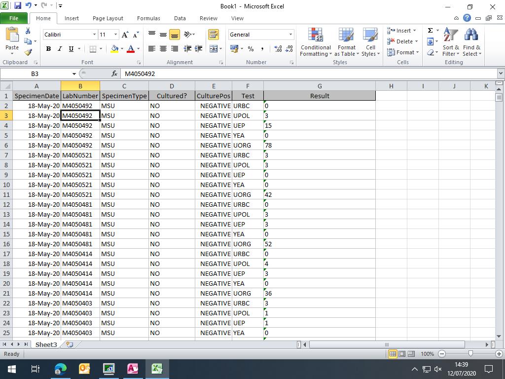
The topic ‘Excel wizards help please!’ is closed to new replies.